| Species | Common name | Family | Broad taxon | Prey family | DL | MFU | MV1 1/3 | MV1 2/3 | MV1 3/3 |
|---|---|---|---|---|---|---|---|---|---|
| Megaptera novaeangliae | humpback whale | Balaenopteridae | baleen whale | invert | 9 | 14 | 17 | 12 | 3 |
| Phocoena phocoena | harbor porpoise | Phocoenidae | dolphin/porpoise | fish | 2 | 4 | 11 | 6 | 1 |
| Stenella coeruleoalba | striped dolphin | Delphinidae | dolphin/porpoise | fish | 0 | 2 | 22 | 3 | 1 |
| Lagenorhynchus obliquidens | Pacific white-sided dolphin | Delphinidae | dolphin/porpoise | fish | 4 | 20 | 40 | 8 | 5 |
| Balaenoptera acutorostrata | minke whale | Balaenopteridae | baleen whale | invert | 1 | 1 | 1 | 2 | 0 |
| Ziphius cavirostris | goose-beaked whale | Ziphiidae | beaked whale | squid | 2 | 2 | 6 | 1 | 0 |
| Phocoenoides dalli | Dall’s porpoise | Phocoenidae | dolphin/porpoise | fish | 6 | 5 | 44 | 8 | 1 |
| Eschrichtius robustus | gray whale | Eschrichtiidae | baleen whale | invert | 0 | 3 | 3 | 1 | 1 |
| Balaenoptera physalus | fin whale | Balaenopteridae | baleen whale | invert | 4 | 16 | 26 | 4 | 2 |
| Berardius bairdii | northern giant bottlenose whale | Ziphiidae | beaked whale | squid | 0 | 2 | 6 | 3 | 0 |
| Balaenoptera musculus | blue whale | Balaenopteridae | baleen whale | invert | 1 | 1 | 6 | 0 | 0 |
| Orcinus orca | killer whale | Delphinidae | dolphin/porpoise | fish | 2 | 3 | 8 | 0 | 1 |
| Grampus griseus | Risso’s dolphin | Delphinidae | dolphin/porpoise | fish | 5 | 3 | 10 | 1 | 2 |
| Balaena mysticetus | bowhead whale | Balaenidae | baleen whale | invert | 0 | 1 | 0 | 0 | 0 |
| Lissodelphis borealis | northern right whale dolphin | Delphinidae | dolphin/porpoise | fish | 4 | 0 | 0 | 0 | 0 |
| Mesoplodon stejnegeri | saber-toothed whale | Ziphiidae | beaked whale | squid | 0 | 0 | 2 | 0 | 0 |
Using spatially explicit models to improve sampling of rare marine species: species-specific behavior and ecology drive depth distribution of cetacean eDNA in pelagic marine environments
- School of Aquatic and Fishery Sciences, University of Washington, Seattle, WA, USA
- Centre for Research into Ecological and Environmental Modelling, School of Mathematics and Statistics, University of St Andrews, St Andrews, Scotland
- School of Marine and Environmental Affairs, University of Washington, Seattle, WA, USA
- Biomathematics and Statistics Scotland, Dundee, UK
- UK Centre for Ecology and Hydrology, Lancaster Environment Centre, Lancaster, UK
- Scripps Institution of Oceanography, University of California San Diego, San Diego, CA, USA
- Northwest Fisheries Science Center, National Marine Fisheries Service, National Oceanic and Atmospheric Administration, Seattle, WA, USA
*Corresponding author email: avancise@gmail.com
Running page head: Depth distribution of rare target detections
Abstract
Detecting rare species is a long-standing challenge in ecological studies that is exacerbated for many marine species due to their remote habitats and elusive behaviors. Environmental DNA (eDNA) sampling is a powerful standalone or complementary tool that promises to improve spatiotemporal models of species’ distribution and abundance, but positive detections of rare species remain difficult to obtain. Targeting optimal sampling depths can improve the detection rates of cetaceans, which are highly mobile and have species-specific depth ranges spanning the surface to 3 km. In this study, we examine the depth distribution of eDNA detections from 16 cetacean species in the California Current Ecosystem using systematic eDNA samples collected from the surface to 500 m. We sequenced five replicates each of 516 samples from 175 unique geographic locations and up to 5 depth strata, obtaining 468 positive cetacean detections across 2,580 sequencing replicates. Given the presence of cetacean eDNA in a sample, we found that the probability of detecting that eDNA using genetic metabarcoding was driven by primer specificity, technical replication, and the number of freeze/thaw cycles a sample was subjected to. Futher, species-specific eDNA detection rate varied with depth and generally reflected known species-specific use of the water column, but could also be modeled using information on taxonomy or diet. Most dolphin and porpoise species had highest predicted detection rates at the surface, whereas most baleen whale species had highest detection rates at the surface in regions close to shore and at 500 m off the continental shelf. Beaked whales had highest detection rates between 300 and 500 m, and were unlikely to be detected on the continental shelf. The depth maximizing detection rate for each species was not geographically consistent, indicating species-specific geographic variability in depth distribution. Our results indicate that the challenge of detecting cetacean species using eDNA can be mitigated in the experimental design phase by using niche-based or spatial distribution models to inform sampling strategies, especially sampling depths. eDNA sampling strategies for cetaceans should account for species-specific depth distributions and habitat use to optimize detection rates; incorporating depth-informed sampling may increase detection rates over non-depth-targeted surveys and strengthen our ability to estimate marine mammal distribution and abundance.
Introduction
Detecting rare species is a longstanding challenge in many ecological fields, e.g., ecosystem-level studies of biodiversity or community composition (e.g., Cao et al., 2001, 2001; Jeliazkov et al., 2022; Queheillalt et al., 2002; White et al., 2023) as well as species-level studies of spatial ecology (e.g., Engler et al., 2004; Guisan et al., 2006; Le Lay et al., 2010). Many methodological approaches have been developed to address this problem, both in the experimental design phase (Guisan et al., 2006; Le Lay et al., 2010) and in the data analysis phase (Engler et al., 2004; Guélat & Kéry, 2018; Lyet et al., 2013). Recently, environmental DNA (eDNA) has emerged as a viable tool for detecting rare species, with promise to improve spatial distribution models (SDMs) and biodiversity monitoring (e.g., Afonso et al., 2024; Valdivia-Carrillo et al., 2025), particularly when integrated with existing survey methods (e.g., Claver et al., 2025; Shelton et al., 2022).
While eDNA-based species detection is a promising approach to estimating or predicting the abundance and distribution of rare species, it may be limited by the collection of point samples of relatively small amounts of water (generally 1-10 L) throughout the study area. This necessitates careful consideration of the inferential aims of the study when deciding where to collect samples to determine species presence/absence or describe geographic (\(x\) and \(y\)) distribution, either independently of or alongside depth (\(z\)) distribution. On the other hand, explicitly sampling across the \(z\) dimension, which is often ignored in marine mammal monitoring programs, will enhance our capability to describe spatiotemporal variability in \(z\) habitat use that, when combined with variability in \(xy\) habitat use, may provide novel insight into the spatiotemporal ecology of these species in three dimensions to inform both the management of rare species and future sampling designs based on 3D ecological behaviors.
Marine mammals, and specifically cetaceans, are notably some of the rarest species in the marine environment in terms of in terms of their relative abundance and the patchiness of their distribution, with estimates of cetacean density (e.g., Becker et al., 2020; Paiu et al., 2024) several orders of magnitude smaller than that of fishes, plankton, or microbes (e.g., Bar-On et al., 2018; Irigoien et al., 2014; Whitman et al., 1998) and decreasing with individual biomass as predicted by ecological theory (Jennings et al., 2008). Traditionally, cetacean habitat use and distributions are mapped using observations from visual and/or passive acoustic surveys (Becker et al., 2022; e.g., Dalpaz et al., 2021; Fiedler et al., 2023; Findlay et al., 1992; Forney & Barlow, 1998; Kanaji & Miyashita, 2021). Visual line transect surveys are the most common, in which observers on board a ship or airplane record detected marine mammals and their distance to the transect line, covering the survey area in a systematic pattern. These surveys are limited to surface (typically <10 m) observations, where most cetaceans spend very little of their time, made in a relatively small radius from the observation platform [e.g., approximately 11 km from a typical NOAA survey vessel; Barlow (2016)], and during daylight hours - and their effectiveness decreases in poor weather or sea state. Ship-based passive acoustic line-transect surveys tow hydrophones along similar systematic transects, and can detect mid-to-high frequency signals within a radius of 10 km, and lower frequency signals in a radius of 10s-100s of km. Static passive acoustic data collection employs hydrophones mounted to surface buoys or the seafloor, with similar detection frequencies and sensitivities. Passive acoustic surveys are not limited to surface or daylight observations, but only detect species that are actively vocalizing.
Systematic eDNA surveys, where water samples are collected along transects, do not share limitations related to depth, daylight, weather conditions, or species’ vocal activity and are therefore potentially powerful as standalone or complementary monitoring tools (Pikitch, 2018). However, it is important to consider the unique limitations of eDNA surveys when using this approach independently or jointly with other methods. Because eDNA survives for several hours to days (Brandão-Dias et al., 2025), an eDNA sample represents a longer temporal integration of species’ occurrence at a given location than visual or acoustic snapshots. Additionally, the distribution of eDNA is influenced by diffusion and transport associated with oceanographic processes (Brasseale et al., 2025; Xiong et al., 2025; Yamahara et al., 2025), as well as sinking rates, and therefore eDNA detected in a sample may have a provenance up to 10s of km from the sample site (Andruszkiewicz et al., 2019). Despite this temporal persistence and potential for movement, eDNA has been previously shown to reflect geographic distributions and depth patterns of marine species (Canals et al., 2021; Guri et al., 2025; Shelton et al., 2022).
Marine surveys are expensive and logistically challenging, and eDNA samples represent a small volume of water (typically <3 L per sample) compared to the survey area. They are also costly to process, so studies targeting a specific set of rare species may benefit from restricting their range of sampling depths via spatial or niche-based modeling. There is currently a lack of published data regarding optimal sampling depths to target rare taxa, or what ecological and observational processes may drive variability in the probability of detecting those taxa across depths.
Here, we first quantify the probability of detecting cetacean eDNA present in a sample, then describe the \(z\) distribution of cetacean species’ eDNA in the water column and use the results to identify broad ecological drivers of observed patterns. We specifically ask:
- Does probability of detection (POD) of cetacean eDNA vary in response to technical replication (Ficetola et al., 2015), primer specificity (Shaffer et al., 2025), or post-extraction DNA degradation (Brandão-Dias et al., 2025) due to laboratory freeze/thaw cycles?
- Does detection rate of cetacean eDNA vary in the depth (\(z\)) dimension? If so, can this variability be predicted by preferred prey categories or phylogeny (e.g. taxonomic family)?
- Does latitudinal and longitudinal variability in eDNA distribution interact with depth variability to affect species-specific detection rate in three dimensions?
To answer these questions, we leverage an opportunistic set of eDNA samples collected from seawater in the California Current in 2019 in order to assess the abundance of North Pacific hake (Merluccius productus). We examine cetacean detections generated via genetic metabarcoding of three mitochondrial target regions. We first use an occupancy model implementend in a hierarchical Bayesian framework to examine the POD of cetacean DNA given it’s presence in an eDNA sample. Next, we use a GAM framework to examine species-specific detection rate across sampling depth (0-500 m), then incorporate spatial location information to examine species-specific variability in detection rate in three dimensions.
Methods
Sample Collection
We used eDNA samples collected on the 2019 US-Canada Integrated Ecosystems and Acoustics-Trawl Survey for Pacific hake from 2 July to 19 August 2019. The study area is within the California Current System, which is 500-800 km wide, extends from 43°N to 23°N, and comprises an equatorward surface current and a subsurface poleward current that is concentrated mainly on the continental shelf (Hickey, 1979). The system is characterized by strong alongshore advection, upwelling concentrated primarily along the continental shelf break, and multiple terrestrial and oceanic water sources (Auad et al., 2011; e.g., McClatchie, 2014). These complex oceanographic processes support a highly productive and diverse assemblage of plankton and fishes, and form a rich prey base for at least 25 cetacean species that inhabit the study area (Carretta et al., 2023).
A full description of field sampling and DNA extraction methods are provided in Shelton et al. (2022). Briefly, we used seawater samples collected at 175 stations in the study area, spanning south-north from latitudes 37.89499°N to 48.39881°N and west-east from longitudes 126.4298°W to 122.8638°W. We targeted five depths for sample collection, so that our sample set of 516 samples included 148 samples collected at the surface (~3 m), 147 samples collected at 50 m, 74 samples collected at 150 m, 73 samples collected at 300 m, and 74 samples collected at 500 m. Where the bottom was shallower than the target sample depth, we did not collect a water sample. The field team collected water using Niskin bottles attached to a CTD rosette and filtered 2.5 L of water from each station and depth using a 47-mm diameter mixed cellulose ester (MCE) filter with a 1-µm pore size and a vacuum filtration manifold connected to a vacuum pump, then immediately preserved the filters in Longmire’s buffer and stored them at room temperature until extraction.
Sample Processing
DNA was extracted using a phase-lock phenol chloroform method as described in Ramón-Laca et al. (2021). We randomized stations and depths across 96-well working plates, removed one plate at a time from the freezer for PCR amplification and library preparation, and stored samples in a -20°C freezer when not in use. Each time we removed a plate from the freezer, we recorded a freeze/thaw cycle for that plate in order to examine the effect of expected DNA degradation due to freeze/thaw cycles on downstream probability of detecting rare species.
We tested all samples for inhibition with quantitative PCR (qPCR) using a Taqman probe assay that included an internal positive control (IPC) of known concentration. We identified inhibited samples by examining the IPC concentration, as described in Shelton et al. (2022). For each sample, we selected a dilution that was determined from the qPCR data (described above) to be not inhibited, which was either 1x or 0.2x across all samples.
We then amplified each sample with three different mitochondrial metabarcode primer sets: MiFish-U (MFU) targeting fishes using the mitochondrial 12S region (Miya et al., 2015), MarVer1 (MV1) targeting all vertebrates using the mitochondrial 12S region, (Valsecchi et al., 2020), and Dlp1.5/Oordlp4 (DL) targeting only cetaceans using the mitochondrial control region (Baker et al., 2018). For all samples, we ran one technical PCR replicate for MFU, one for DL, and three for MV1. We optimized primer, Taq, and cycling conditions using mock communities (Shaffer et al., 2025).
Our reaction mixture for amplification (PCR1) consisted of 10 μL of Phusion Master Mix (2X), 0.4 μL of the forward primer (10 μM); 0.4 μL of the reverse primer (10 μM), 0.6 μL of 100% DMSO, 0.5 μL of rAlbumin (20 μg/μL), 4.4 μL of nuclease-free water and 2 μL of DNA template. We ran PCR1 with the following cycling conditions: an initial denaturation of 98°C for 30 sec; followed by cycles of: denaturation (98°C for 10 sec), annealing (60°C for 30 sec), and extension (72°C for 3 sec); with a final extension of 72°C for 10 min and hold at 4°C. We ran 35 cycles for MFU and MV1, and 40 cycles for DL.
If a sample failed to produce a band at the previously determined optimal dilution when amplified using MV1 or MFU, we diluted the sample and reran it until a visible band was produced. We could not do the same for DL, which targets only cetaceans, because the rarity of our target made it prohibitively difficult to distinguish between an inhibited sample and a negative sample. Here we assumed that the optimal dilution selected by qPCR was not inhibited and treated samples without bands as negative detections.
Any MFU and MV1 samples that returned fewer than 1000 classified non-human reads after sequencing were rerun in an effort to complete the dataset to include one successful MFU replicate and three successful MV1 replicates. This required up to six replicate sequencing runs in some cases.
Library Preparation and Sequencing
We then cleaned the amplified PCR product using Ampure Beads (1.2x beads:product ratio, with two 70% ethanol washes) and indexed each sample in a second PCR reaction (PCR2) using the following reaction mixture: 12.5 μL of KAPA HiFi HotStart ReadyMix (Roche Diagnostics), 1.25 μL of IDT for Illumina DNA/RNA UD Indexes (Sets A-D), as well as primer-specific volumes of PCR1 product and nuclease free water. We added 5 μL PCR1 product, and 6.25 μL of nuclease free water for all MFU and MV1 samples, and added 11.25 μL PCR1 product and no nuclease free water to all DL samples. We ran PCR2 using the following cycling conditions: an initial denaturation of 95°C for 5 min; cycles of: 98°C for 20 sec, 56°C for 30 sec, 72°C for 1 min; and a final extension of 72°C for 5 min. We ran eight cycles for MFU and MV1, and 12 cycles for DL.
After indexing, we visualized the PCR product on a 2% agarose gel and quantified DNA concentration using Quant-iT™ dsDNA Assay Kit (Thermo Fisher Scientific, USA) with Fluoroskan™ Microplate Fluorometer (Thermo Fisher Scientific, USA). We then pooled equal quantities of DNA product from each sample into 96-sample libraries for sequencing, and extracted the target band using the E-Gel™ SizeSelect™ II Agarose Gels (Thermo Fisher Scientific, USA). Finally, we loaded our pooled libraries, in 6-8 pM concentrations with a 20% PhiX spike-in, onto an Illumina MiSeq platform at the University of Washington with a v3 600 cycle kit. In total, we ran 36 sequencing runs between May 2023 and July 2025.
For every sequencing run, we added a sample with nuclease-free water (negative control) and genomic DNA from kangaroo (positive control) to PCR1 and carried it through the rest of the library preparation workflow. If anything other than human or NA was found in the negative control, or if kangaroo appeared in any other eDNA sample, we omitted that plate from the final analysis. This occurred for only one plate of technical replicates, which were removed from downstream analyses.
Bioinformatic Processing
We analyzed all sequencing data using the bioinformatics workflow established in Guri et al. (2025). We trimmed Illumina-demultiplexed reads with Cutadapt v4.9 to remove primer and adapter sequences, allowing a maximum mismatch rate of 0.1 (Martin, 2011). We then conducted quality filtering and minimum-length truncation using DADA2, and inferred amplicon sequence variants (ASVs) using default denoising settings (Callahan et al., 2016).
Following initial QAQC of the raw sequence data, we queried each unique ASV against a vertebrate mitochondrial subset of the January 2025 NCBI nr eukaryote database using standalone BLAST configured with “-word_size 20 -evalue 1e-30 -max_target_seqs 100” (Altschul et al., 1990), supplemented with a negative-taxid file to remove taxa that are not known to occur in the North Pacific Ocean. We also excluded psuedogenes and unverified predicted or modeled sequences, i.e., sequences with accession IDs beginning in XM or XR. We made taxonomic assignments using a least-common-ancestor procedure in TaxonKit v0.17 (Shen & Ren, 2021), prioritizing exact-identity matches and otherwise accepting a match threshold of >99.3% (1 locus mismatch). In cases where multiple species met this criterion, we assigned the sequence to its least common ancestor. After classification, we manually reviewed all cetacean identifications to ensure consistency with regional species distributions.
Detection Data QAQC
After bioinformatic processing of all samples, we removed any additional dilutions of MFU or MV1 samples that were run to maximize sequencing success, keeping only the iteration with the greatest total read count. We then defined a sample as a station/depth/technical replicate combination. To obtain positive detections for each sample, we kept any species with > 1 sequencing read. We filtered out any non-target (non-cetacean) species, and also removed detections of bottlenose dolphins, which we considered likely contamination from concurrent labwork focused on this species, and unidentified Balaenopterids or Delphinids. Across all samples, we define non-detection as 0 reads for a given cetacean species in a station/depth location that was positive for non-target species (e.g. fish) in either MFU or MV1 sequence data.
Data Analysis
Question 1: How does observation error affect POD of cetacean DNA?
The decisions made during sample collection, processing, and sequencing can introduce observation error. We therefore used the information contained in multiple technical replicates from individual biological samples to better understand the detection processes for cetacean eDNA. Here we estimate the probability of detection (POD) of cetacean DNA from any species, under the assumption of an equal POD across all cetacean species’ DNA if it is present in the sample, which approximates empirical results for the primers used in this study (Shaffer et al., 2025). We used a Bayesian hierarchical occupancy model to separately estimate the probability of occupancy/capture by depth and POD by primer and number of freeze/thaw cycles, based on the model presented in Patin et al. (in review).
We modeled the presence of cetacean eDNA at site \(i\) and depth \(z\), \(w_{i,z}\), as a Bernoulli random variable with occurrence probability \(\Psi_z\):
\[ w_{i,z} \sim \text{Bernoulli}(\Psi_{z}) \]
where probability of presence in a sample at depth (\(\Psi_z\)) is given as the logistic transform of an intercept (\(\beta_0\)) plus a smooth function, \(f\), of sample depth \(z\):
\[ \text{logit}(\Psi_z) = \beta_0 + f(z). \tag{1}\]
We then modeled the observed detection of cetacean eDNA in each technical replicate \(d_r\) as a Bernoulli random variable with primer- (\(m\)) and freeze/thaw-specific (\(t\)) POD \(\Omega_\text{m*t}\) conditional on presence in the biological sample \(w_{i,z}\):
\[ d_r \sim \text{Bernoulli}({\Omega_\text{m*t}} \cdot w_{i,z}). \tag{2}\]
where POD (\(\Omega\)) is a logit-linear function of primer type (\(m\)) and number of freeze/thaw cycles (\(T\)) that the sample used for the technical replicate \(r\) has been subjected to:
\[ \text{logit}(\Omega_{m*t}) = \gamma_m + \gamma_t \cdot T_r. \tag{3}\]
Here, \(\gamma_\text{m}\) is a primer-specific intercept and \(\gamma_\text{t}\) is a slope parameter that interacts with \(T\), the number of freeze/thaw cycles.
We implemented this model using nimble [de Valpine et al. (2017); zenodo.17954119] in R (R Core Team, 2016). We used uninformative or weakly informative prior distributions for model parameters and ran four chains, each with 250,000 iterations, 225,000 of which were burnin, and assessed convergence using the Gelman-Rubin diagnostic (Gelman & Rubin, 1992).
Using the posterior mean estimates of detectability after one freeze-thaw cycle, we simulated the primer-specific expected detectability with increasing technical replication while holding freeze-thaw cycles constant.
We were not able to model species-specific \(z\)-distribution of eDNA detectability using the occupancy model because models with species-specific smooths on depth did not converge; we hypothesize that this was due to model overparameterization relative to the amount of data available per species (particularly the number of positive detections). We therefore visually compared the predicted \(z\)-distribution of cetacean eDNA in an occupancy framework vs. a generalized additive model (GAM) framework to confirm that both models produced qualitatively similar estimates of the \(z\)-distribution of cetacean DNA, and used GAM models for Questons 2 and 3 in our study.
Question 2: Does species-specific POD vary with depth?
For all following analyses, we define detection rate as the probability of detecting cetacean eDNA in a sample without the assumption of its presence in the sample, so that species-specific detection rate comprises both the probability of that species’ occurrence at a site as well as the probability of capturing and detecting the species’ eDNA in a sample. Because cetacean DNA POD varies only minimally across cetacean species for the primer sets used in this study (Shaffer et al., 2025), we interpret variability in detection here to be driven primarily by variability in the distribution of species-specific eDNA. Similarly, we have excluded primer specificity, technical replication, and number of freeze/thaw cycle from downstream analyses to ensure model convergence; these were applied randomly across biological samples to minimize bias in observation error.
To determine whether species-specific detection rate varies in the \(z\) dimension, we applied generalized additive models [GAMs; S. N. Wood (2017)] as implemented using the mgcv package in R (R Core Team, 2016). GAMs have previously been demonstrated to be an appropriate tool for modeling spatial distributions of cetaceans (Abrahms et al., 2019; e.g. Becker et al., 2022). Our binomial response was the detection or non-detection at each combination of site, depth, and technical replicate. Models were constructed with increasing complexity; in each a case a smooth effect of depth was used, but allowing for structure including taxonomy or preferred prey. Models were defined as follows:
\[ \begin{align} \text{logit}(\mu(z)) = &\beta_0 + f(z) \quad \text{(depth smooth)}\\ \text{logit}(\mu(z,s)) = &\beta_{s} + f(z) \quad \text{(depth smooth, species intercept)}\\ \text{logit}(\mu(z,s)) = &\beta_{s} + f_s(z) \quad \text{(depth smooth varying by species)}\\ \text{logit}(\mu(z,F)) = &\beta_{F} + f_F(z) \quad \text{(depth smooth varying by family)}\\ \text{logit}(\mu(z,e)) = &\beta_{e} + f_e(z) \quad \text{(depth smooth varying by prey)} \end{align} \tag{4}\]
Here \(\mu\) is the detection probability for a cetacean in a sample, its arguments indicate its functional dependence. In each case \(f\) denotes a smooth function, modelling by a spline, \(f_X\) indicates a factor-smooth (Pedersen et al., 2019) of depth and species (\(s\)), family (\(F\)) or preferred prey (\(e\)). \(\beta_0\) is a shared intercept parameter and \(\beta_X\) is an intercept parameter per level in \(X\) where the convention for the factor-smooths is followed. In all cases \(z\) is depth.
We assessed model fit using AIC, and model performance using standard metrics including the percent of deviance explained, the area under the receiver operating characteristic curve (AUC, Fawcett, 2006), the true skill statistic (TSS, Allouche et al., 2006), and a visual comparison (i.e. via plotting) of predicted vs. observed detection rates across sampling depths. We also visually compared our model-based predictions of probability of detection across depth with estimates of species-specific time-at-depth as reported by Watwood and Buonantony (2012) and the U.S. Department of the Navy (2017).
Question 3: Does depth variability in detection rate vary spatially?
We also used a GAM to examine spatial variability in the detection rate across depths. We approach this question in two ways: first, we examining variability in the effects of depth, latitude, and longitude on species-specific detection rate; next, we examine variability in the effects of depth and species-specific predictions of density on species-specific detection rate. We used the best fitting model from Question 2 as our starting point (species-specific variability in detection rate with depth), subset our input data to include the species from each broad taxon with the greatest number of detections, and pulled predicted density values for our survey area from Becker et al. (2020), which are predicted based on >25 years of visual sighting data.
For approach 1, we looked species-specific variation in spatial-depth smooths with the following model formulation:
\[ \text{logit}(\mu(x,y,z,s)) = \beta_{s} + f_s(x,y,z). \tag{5}\]
Here \(f_s(x,y,z)\) was constructed as tensor product of marginal smoothers of \(x\), \(y\), and \(z\) and in the case of the species-specific factor-smooth interaction we used the tensor product of \(x\), \(y\), and \(z\), and a random effect on species. We constructed intermediate tensor products on interactions among all three spatial variables and species (using the ti() constructor in mgcv; S. N. Wood (2017), Section 4.6.2). This allowed us to decompose the smooth of space and depth as:
\[\begin{align} f_s(x,y,z) = &f(x,y) + \quad \text{(spatial only)}\\ &f(z) + \quad \text{(depth only)}\\ &f_s(x,y) + \quad \text{(per taxon spatial)}\\ &f_s(z) + \quad \text{(per taxon depth)}\\ &f_s(x,y,z) + \quad \text{(full interaction)}\\ &\beta_s \quad \text{(species random effect)}, \end{align}\]
where \(\beta_s \sim N(0,\sigma_s)\) is a random intercept per species, \(f\) indicates a smooth of the variables, and \(f_s\) indicates a factor-smooth interaction between the variables in the function’s argument and species. When \(x\) and \(y\) are included in a model, their effect was constructed as a bivariate thin place spline on these projected coordinates (since they would obey the isotropy property). Interactions between space and depth required a tensor product (as moving one unit in depth is not the same as one unit in space).
For approach 2, we looked for variability in depth \(z\) and predicted species density \(D\) on a species-specific basis with the following model formulation:
\[ \text{logit}(\mu(i,z,s) = \beta_{s} + f_s(z) + f_s(D_s(x_i,y_i)) \tag{6}\]
where \(f(z)\) is a smooth of depth, common across all species and \(f_s(D_s(x,y))\) is constructed as independent smoothers with one smooth for each species (level of \(s\)). \(D_s(x_i,y_i)\) is the predicted density (animals per kilometre) for species \(s\) at location \(x_i,y_i\) of site \(i\) as taken from Becker et al. (2020). \(\beta_s\) is a per-species intercept.
As in Question 2, we assessed model fit using AIC, and model performance for the best model using percent deviance explained, AUC, and TSS. We then conducted a visual comparison of the predicted depth of maximum detection rate across and observed detection depths within the study area for the most frequently observed baleen whale, dolphin/porpoise, and beaked whale.
A table of all variables used in both the occupancy model and the GAM framework is included in the Supplementary Materials (Supplemental Table S2).
Results
We selected 516 water samples collected at 175 unique locations during the 2019 NOAA hake abundance survey (Figure 1), targeting surface, 50, 150, 300, and 500 m sampling depths at each station. We amplified and sequenced these samples in 1 technical replicate using MFU, 3 technical replicates using MV1, and 1 technical replicate using DL, resulting in a final total of 1548 successfully amplified and sequenced samples.
Across all samples, we observed 468 positive detections of 16 cetacean species, including 6 baleen whale species, 5 dolphin species, 2 porpoise species, and 3 beaked whale species (Table 1). 11 species were observed more than 10 times, and and additional 5 were observed fewer than 10 times. We also detected bottlenose dolphins (Tursiops truncatus) a total of one time in the dataset; this detection occurred north of the known range of this species in the California Current (Carretta et al., 2024). As noted in the methods section, we consider this detection likely to have resulted from lab contamination and removed it before downstream processing.
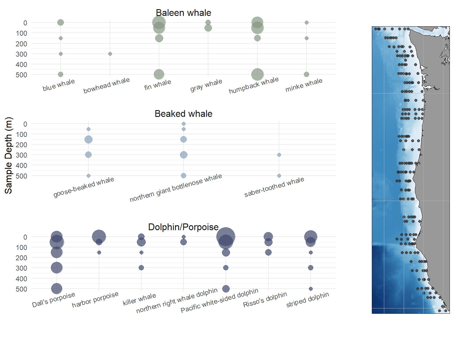
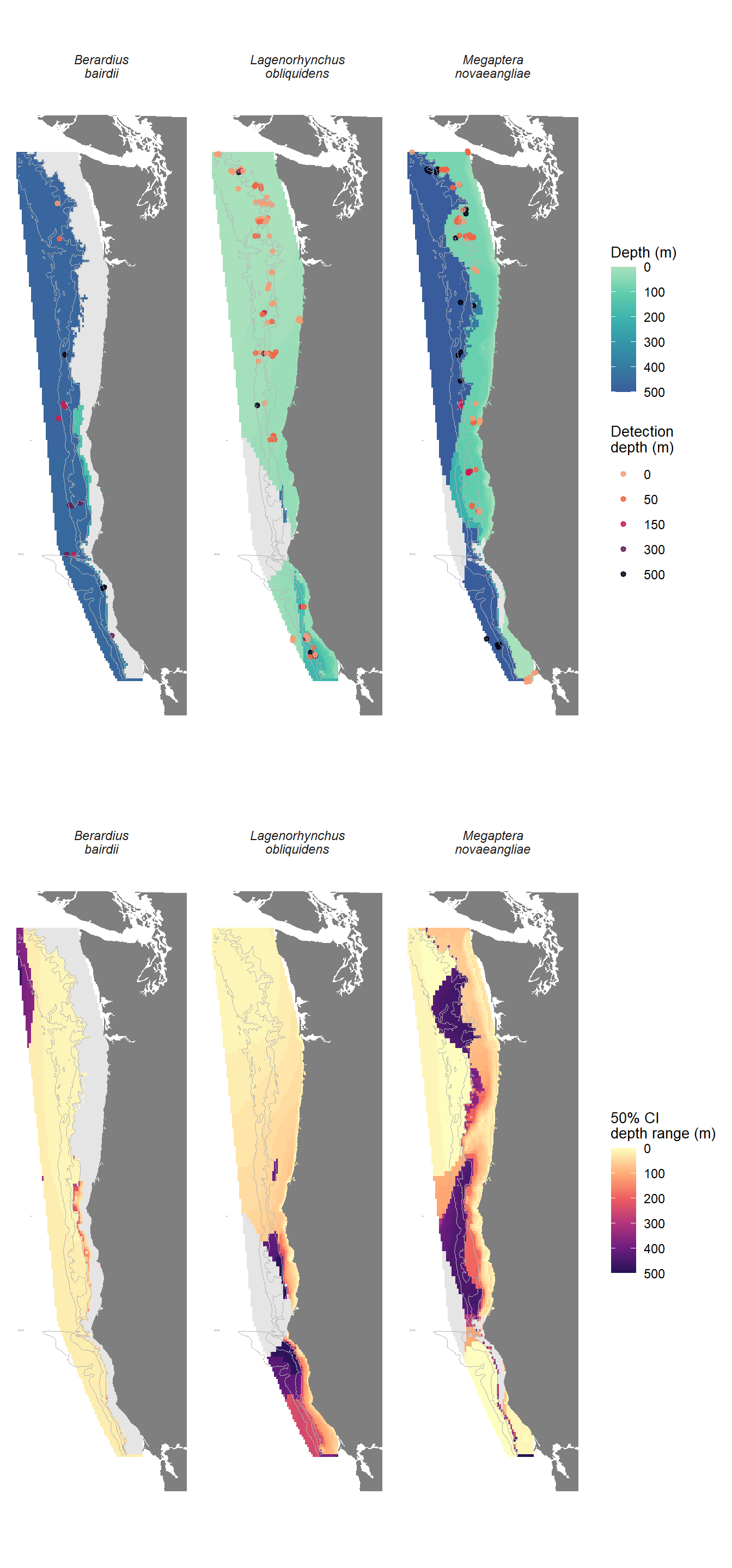
Figure 1 illustrates the distribution of detections across sampling depths \(z\), ignoring \(xy\) distribution, for all cetacean species included in the study. Notably, our dataset includes one unexpected detection of a bowhead whale (Balaena mysticetus), not generally observed south of 63 N latitude in the Bering Sea since the end of commercial whaling and not known to ever inhabit the California Current (Rugh et al., 2003), as well as three detections of extremely rare saber-toothed whales (Mesoplodon stejnegeri), a cold-water beaked whale observed only twice, in the Gulf of Alaska, in 1986-2005 (Hamilton et al., 2009). This is the first direct observation of this species in the California Current to date; it previously was only known to inhabit the region based on two stranding events from May 2015 in Oregon and Washington (Becker et al., 2020; Hamilton et al., 2009; Moore & Barlow, 2017).
Question 1: Quantifying the effect of observation bias on detectability
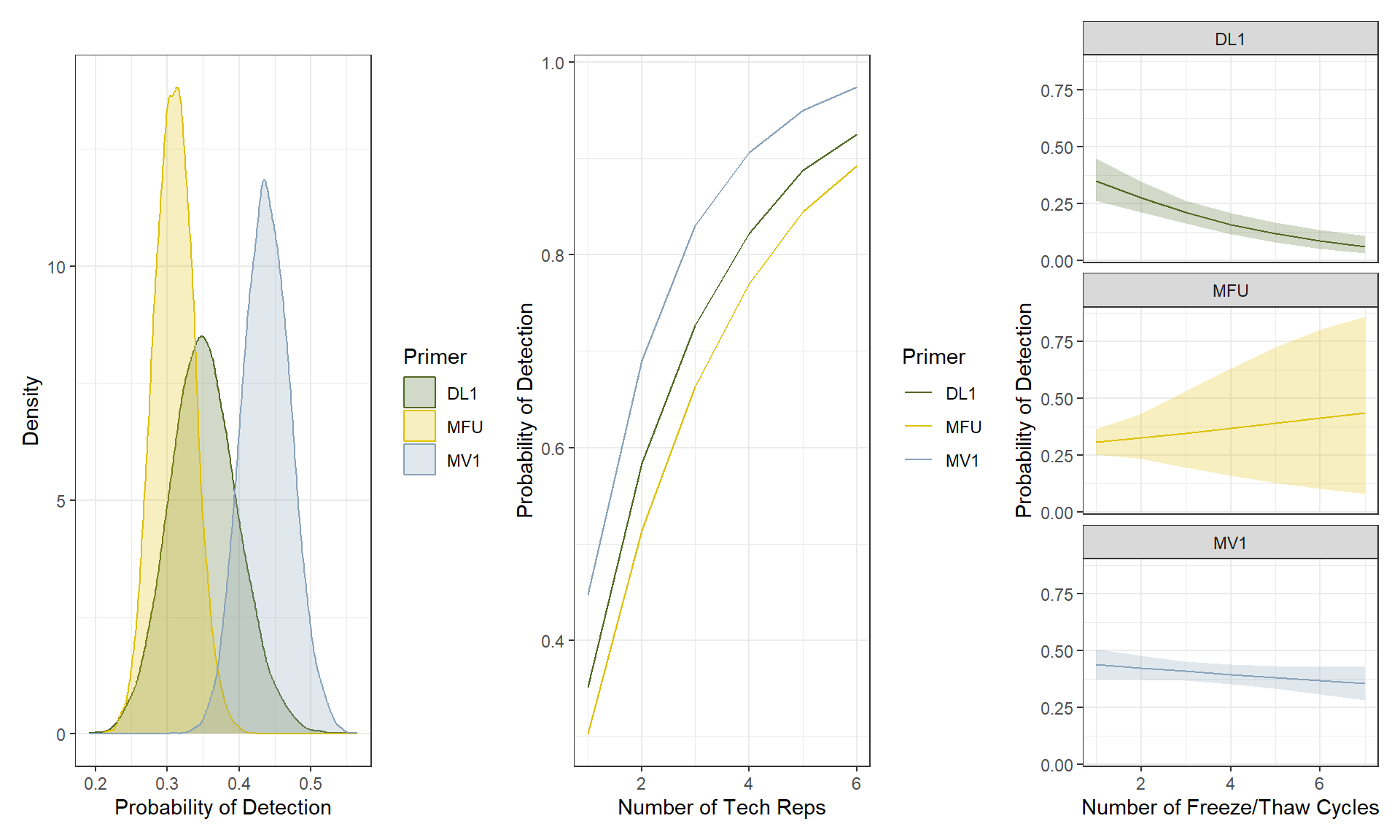
Given the presence of cetacean eDNA in a sample, its POD is affected by primer choice (Figure 2, left). Assuming a single freeze/thaw cycle and technical replicate, MV1 had the highest expected POD (\(\Omega_\text{m*t}\), 0.44), followed by DL (0.35) and then MFU (0.31). Using the mean posterior POD for each primer at one freeze/thaw cycle (\(\Omega_{m*1}\)), we calculated the expected rate of increase in POD with increasing technical replication by primer (Figure 2, middle). Based on our results, achieving a POD >90% for cetacean DNA collected in a sample would require four technical replicates of MV1, ~5-6 technical replicates of DL, or seven technical replicates of MFU.
While increasing the number of technical replicates increases POD, the number of freeze/thaw cycles decreases POD (Figure 2, right), consistent with increased degradation with increasing freeze/thaw cycles. We found a relationship between freeze/thaw cycle and posterior estimates of POD for the longest primer in our study (DL, 360 bp), and a weaker relationship between freeze/thaw cycle and posterior POD for MV1 (202 bp). There was no relationship detected between posterior POD and freeze/thaw cycles for MFU (185 bp), noting limited statistical power to detect the effect of freeze/thaw as only 5 of 516 total MFU samples sequenced in this study had > 2 thaw cycles.
Given our posterior estimates of POD by primer and number of freeze/thaw cycles, we calculated a sample-specific POD for each sample in our study, assuming cetacean DNA is present in the biological sample. Averaged across all samples in this study when accounting for freeze/thaw cycles, the mean detectability for cetacean DNA in a single technical replicate of DL is 0.14, for MFU is 0.31, and for MV1 is 0.39. Despite the significant reduction in POD in our DL sequence with increasing degradation caused by increasing freeze/thaw cycles (lowest DL POD = 0.08), including an additional four replicates using primers that target shorter DNA fragments that were not as strongly affected by freeze/thaw cycle (MV1 and MFU) ensured a high overall POD for cetacean eDNA in a biological sample, conditional on its presence. We estimated the sample-specific predicted DNA POD for each sample in our study using the sample-specific parameters for number of freeze/thaw cycles and primer used in each technical replicate and calculating POD across all technical replicates for each sample combined. Using this approach, we determined that mean predicted POD across all samples in the study was 0.87 (range: 0.85 - 0.92).
Question 2: Does POD vary with depth?
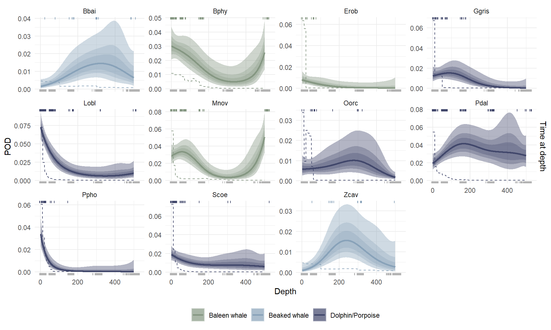
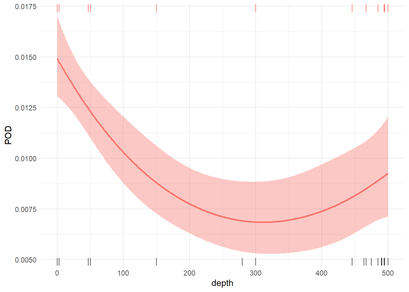
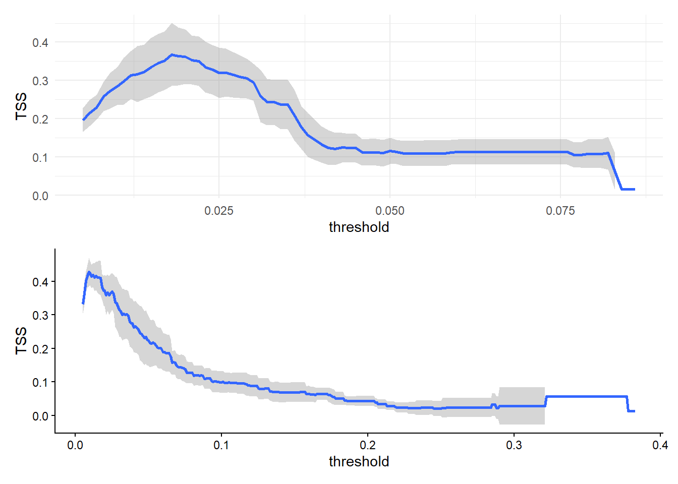
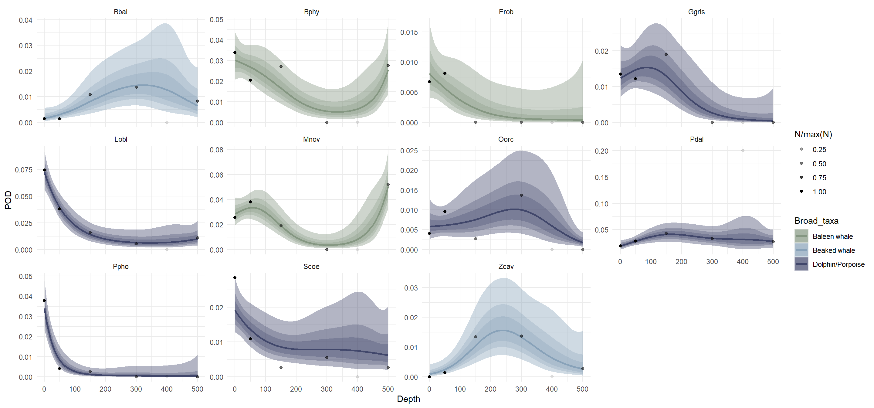
In the next two sections we switch to considering detection rate of cetacean DNA in the ocean using five technical replicates per sample (3 MV1, 1 DL, 1 MFU), without assuming its presence in a biological sample. Detection rate varies with depth (p << 0.001, deviance explained = 0.7%; Supplemental Figure S1); the model that best describes variance in detection rate with depth includes significant smooth terms for depth, species, and a depth x species interaction (AIC = 4547, Table 2). This model explained 14.3% of variance in eDNA detection probability, with a mean AUC of 0.73 and a mean optimized TSS of 0.38. Per-species AUC and TSS values are shown in Supplemental Table S3 and Supplemental Figure S2. Finally, we found general agreement between species-specific model predictions and raw detection data via visual comparison (Supplemental Figure S3).
| Model | Stratification | \(df\) | \(Δ AIC\) |
|---|---|---|---|
| \(β_s + f_s(z)\) | species | 48.0 | 0.0 |
| \(β_s + f(z)\) | species | 19.3 | 141.6 |
| \(β_s + f_F(z)\) | family | 19.7 | 307.4 |
| \(β_s + f_e(z)\) | prey | 13.2 | 412.5 |
| \(β_0 + f(z)\) | none | 3.7 | 549.4 |
Broadly, delphinid detection rate was highest at the surface, beaked whale detection rate was highest at depths > 200 m, and baleen whale detection rate was highest either at the surface or at depths > 400 m (Figure 3). Note that although detection data from the five species detected fewer than 10 times were included in our model input, we did not make predictions for any of these species.
Among the delphinids, species-specific trends in detection rate generally reflected previously developed estimates of time-at-depth (U.S. Department of the Navy, 2017; Watwood & Buonantony, 2012). Conversely, most beaked whale and baleen whale species in the study were very likely to be detected outside depths where they were estimated to spend most of their time (Figure 3). Most notably, predicted detection rate depth distribuitons for two of the three baleen whales indicated a high detection rate at 500 m, while these two species spend most of their time above ~200 m depth. Per-species model predictions are shown alongside observed detections in Supplemental Figure S5.
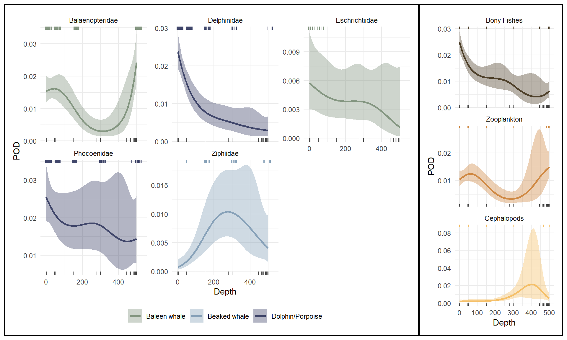
Models stratifying detections by taxonomic family and preferred prey type both had lower AIC values than the model stratified by species (AIC = 4854 and 4960, respectively); however, these models still had significant terms for family and depth-by-family interactions (taxonomic model) and for depth, prey type, and depth-by-prey type interactions (prey type model). Predicted detection rate curves for each model illustrate varying trends in detection rate with depth across strata (Figure 4). Similar to the model stratified by species, we did not make predictions for families with fewer than 10 detections using the taxonomic model, which excluded the Balaenidae (bowhead whale family).
Question 3: Does depth variability in POD covary with geographic variability?
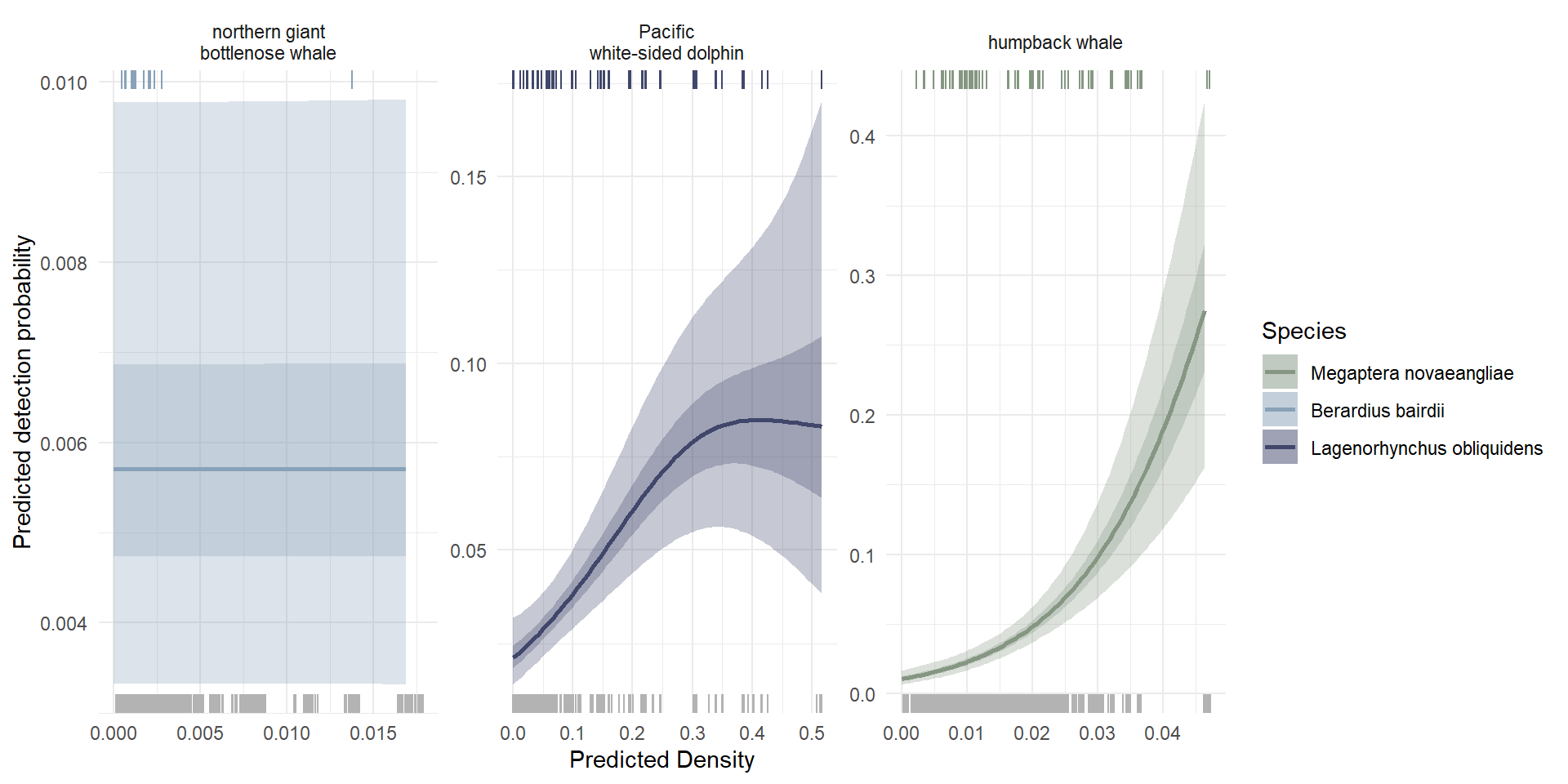
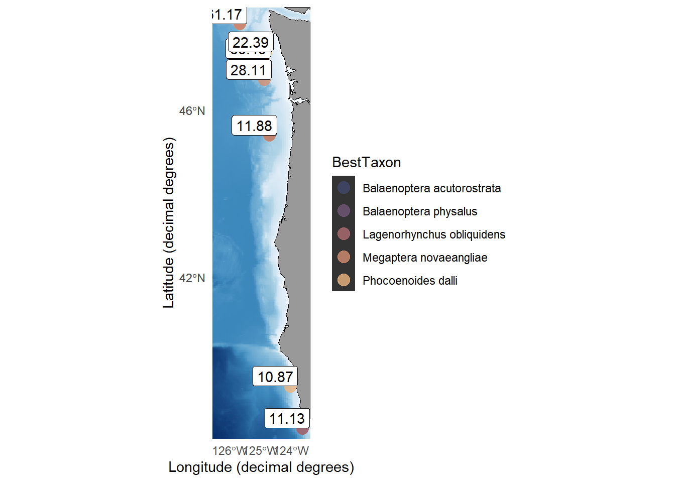
For a subset of the data comprising the most frequently detected delphinid (Pacific white-sided dolphin, Aethalodelphis obliquidens), baleen whale (humpback whale, Megaptera novaeangliae), and beaked whale (northern giant bottlenose whale, Berardius bairdii), we found that covariability in \(xyz\) (AIC = 1410, deviance explained = 26.2%) predicted species-specific detection rate better in our study area than variability in predicted density (\(D\)) and depth (\(z\); AIC = 1571, deviance explained = 10%). Significant terms in our \(xyz\) model included an interaction between species and \(xys\), and interaction between species and \(xy\), and an interaction between species and \(z\). While the unfactoered terms for \(z\) and \(xy\) were not significant, removing these terms increased model AIC to 1413. Mean AUC of our \(xyz\) model across a 10-fold validation test was 0.77 and mean optimized TSS was 0.43. Full model TSS for all thresholds are shown in Supplemental Table S3 and Supplemental Figure S2. Although adding \(xy\) improved model performance, the predicted depth of maximum detection rate for the most frequently detected delphinid, baleen whale, and beaked whale exhibited only marginal variability across \(x\) and \(y\), largely adhering to the broad trends identified in Q2 (Figure 5).
The Pacific white-side dolphin detection rate was maximized near the surface, with maximum detection rate at depths shallower than 100 m in 68% of the study area. The depth of maximum detection rate was deeper toward the south and east of the study area; however, model uncertainty increase in the same region. The predicted detection rate was less than 0.5% in two small regions off near Cape Mendocino, representing approximately 3% of the study area.
The depth that maximized detection rate for northern giant bottlenose whales was greater than 150 m in 52% of the study area, with an additional 31% of the study area where predicted detection rate at all depths less than 0.5%. Notably, the region where predicted detection rate was near zero was along the coastline and continental shelf reagion throughout the study area. Similar to patterns observed for the Pacific white-sided dolphin, the depth of maximum detection rate was deeper to the south and east of the study area, with increasing model uncertainty in the same region.
For humpback whales, there were two disparate peaks that maximized detection rate - above 150 m or below 450m - with no depths between 200 and 400 m maximizing detection rate throughout the study area. The predicted detection rate was maximized at depths shallower than 150 m in 40% of the study rea, mainly along the coast and continental shelf, and wdas maximized at depths greater than 450 in 33% of the study area, mainly along the shelf break and in deeper water. Model uncertainty was greatest for this species along the shelf break representing the transition zone between the two depths, and small outside the transition zone. A small region offshore of Cape Mendocino had predicted detection rates lower than 0.5%, representing 1.5% of the study area.
While our model predicting detection rate across depth and predicted species’ density did not perform as well as our \(xyz\) model, the model included significant terms for the effect of predicted density on detection rate in two of the three species included in this section: Pacific white-sided dolphins and humpback whales. For both of these species, the predicted detection rate increased with predicted species’ density (Figure 6). There was no relationship between predicted species’ density and predicted detection rate for northern giant bottlenose whales within the ranges of predicted species’ densities that were included in our study area (0 - 0.015).
Discussion
Cetaceans are highly mobile and rare among marine species in both abundance and density. Moreover, the distribution of cetaceans throughout the water column spans 100s to 1000s of meters and poorly characterized for many species. eDNA sampling at depth addresses this data gap. Mapping the \(z\) distribution of cetacean eDNA has the potential to provide new insight regarding their 3D spatial use and improve estimates of abundance or distribution, especially for visually or acoustically elusive species. Here we show that the use of occupancy models and niche-based GAMs can inform and optimize eDNA sample collection and processing. For cetaceans and other highly mobile rare marine species, tailoring experimental design based on the results of this study could increase detection rates and improve distributional or abundance models while minimizing cost.
Question 1:
We began with an occupancy model to explicitly separate the effects of cetacean eDNA presence at the sampling site/in the bottle and downstream detection in the sequence data. By implementing this framework we observed an increase in POD with increased primer specificity. Similarly, increasing technical replication increases POD, except that increasing freeze/thaw cycles decreases POD and may counteract the effect of technical replication for longer target regions if technical replicates are not processed concurrently, as was observed with DL in this study. Shorter regions (MFU and MV1) are more robust to decay from freeze/thaw cycles but lower genetic variability in cetacean DNA in each of those regions hinders the ability to classify sequences to species, which necessitated manual curation of the reference database for each of these primers. Within the Delphinidae family, several sequences could not be resolved to species, resulting in the loss of 2 MFU species-level detections and 17 MV1 species-level detections. These family-level detections could not be included in downstream species-specific models of eDNA distribution.
Similar studies have found that observation bias and rare species dropout in eDNA sampling are affected by a number of parameters in the sample collection and processing protocols (Gold et al., 2023; e.g. Shelton et al., 2023), including sampling volume (Patin et al. in review), filter type and pore size (Liu et al., 2024), primer specificity (Shaffer et al., 2025), and technical replication (Ficetola et al., 2015), among others. The results of our study indicate that when present in a sample, rare species can be detected more efficiently using primers with higher specificity and targeting regions with greater variability among the taxa of interest; further, the samples should be subjected to a limited number of freeze/thaw cycles in order to preserve the integrity of longer DNA fragments. Because increased technical replication is advisable to increase detection of rare species DNA in a sample, the best practice would be to conduct all technical replicates for a given sample set concurrently, thus only needing to thaw the extracted DNA 0-1 times before amplification and sequencing.
After accounting for observation bias in our detection rates, we found that predicted cetacean eDNA distribution across depth was qualitatively similar when fitted in an occupancy model context (Eq 1-3) as compared to the non-species specific GAM (Eq 4) in Question 2. Estimates of cetacean POD from the occupancy model were higher overall than detection rate estimates from GAM models, with confidence intervals approaching 1. This is logical given that the Bayesian hierarchical occupancy model estimates POD conditional on the presence of target eDNA in the sample, whereas the GAM did not distinguish POD from the probability of a target species’ occurrence at a sampling site, leading to lower overall detection rate. Continued eDNA sampling at these locations will facilitate the convergence of a fully hierarchical occupancy model with species-specific splines on depth; improving our ability to delineate the effects of observation error (eDNA POD) from ecological processes (eDNA occurrence) in detection rate.
Question 2:
Detection rate across all cetaceans varied with sampling depth (Supplemental Figure S1) and was best described at a species-specific level, broadly reflecting our current understanding of species-specific variability in use of the water column (Figure 3). This was especially evident among the delphinids and porpoises, with some noticeable deviations from expected trends in both the baleen whales and the beaked whales. These trends could be inherent to the behavior of the animals themselves, or more likely may reflect the “behavior” of eDNA.
For example, baleen whales are generally thought to be shallow divers, and while some dives up to approximately 500 m have been recorded in a few species (e.g., fin whales, Panigada et al., 1999), recent reports of time-at-depth for cetacean species indicates that baleen whales spend the vast majority of their time within the top 100-200 m of the ocean (U.S. Department of the Navy, 2017; Watwood & Buonantony, 2012). We observed a sharp spike in detection rate at 500 m for two of the three baleen whale species included in our model predictions. Gray whale eDNA was not likely to be observed at 500 m; this is most likely because they are a nearshore coastal species that is rarely observed over deep water. Humpback and fin whales both have pelagic distributions, and both species’ eDNA was as likely to be observed at 500 m as at the surface, with low detection rates at intermediate depths.
We considered several possible explanations for this observed pattern. We first considered the possibility that some of these deeper eDNA detections, especially those of deeper-diving fin whales, are detections of deep dives made by animals foraging for krill at depth. However, based on our current knowledge of the diving limits of baleen whales, we consider it highly unlikely that most of the deep detections are indicative of the presence of the detected species at that depth. We then considered the possibility that the large spike in deep detections was driven by whale fall or predation (i.e. whole or parts of animals sinking in the water column). In total, baleen whales were detected below 250 m at 28 locations; of those, 8 detections (28.5%) were within 100 m of the ocean floor and might be considered potential detections of whalefall. A map of these detection locations is included in Supplemental Figure S4. In addition to this, a single baleen whale detection coincided with the detection of killer whale eDNA belonging to a potential baleen whale predator. No eDNA detections of baleen whales coincided with the detection of shark eDNA in the data generated from MFU or MV1 sequencing runs.
Finally, we considered the possibility that these deep-water detections are attributable to sinking whale feces. Even after accounting for whale fall or predation events as possible explanations, there remain 19 deep-water detections of baleen whale eDNA (68% of deep-water detections) that are unexplained. While sinking rates and depths of baleen whale feces are generally unknown, we know from expert observations that fecal material from whales is quite large and can sink rapidly from the surface (K.M. Parsons, unpublished observations). Research on oceanic particle sinking rate indicates that smaller particles (up to 6 mm) can sink at rates of ~50-300 m day-1, and that sinking rates increase rapidly with particle size while degradation rates decrease with increasing particle size, with maximum sinking depths in the range of ~800-5,000 m day-1 (Giering et al., 2020; Iversen & Ploug, 2010; McDonnell et al., 2015). eDNA can be detectable for up to 2-4 days at the surface (Brandão-Dias et al., 2025; S. A. Wood et al., 2020), and likely longer at depth where it is colder, darker, and there are fewer microbes digesting cellular material (Andruszkiewicz et al., 2017).
Based on this, the maximum sinking depth of larger poop particles may far exceed the \(z\) range of our study area. It is possible that baleen whale detection rates will continue to increase with increasing depth in some regions due to rapid particle sinking and longer eDNA residency times at depth (Andruszkiewicz et al., 2017). Generally, eDNA is thought to travel 2-20 horizontal km before it is no longer detectable (Andruszkiewicz et al., 2019; Baker et al., 2018; Silva et al., 2025); therefore on a broad scale these detections are likely to reflect the \(xy\) distribution of these species but the temporal resolution of detections may decrease from days to weeks in samples from deeper environments.
Beaked whales were also generally detected deeper than where time-at-depth models predict they spend most of their time (Figure 3), although still within their range of vertical habitat use. Beaked whales spend less of their time near the surface than either baleen whales or delphinids; time-at-depth models estimate that they spend approximately 70% of their time below 100 m (U.S. Department of the Navy, 2017; Watwood & Buonantony, 2012), with depth ranges spanning down as far as 3,000 m (Schorr et al., 2014). While below the surface, beaked whales generally make deep (500+ m) foraging dives interspersed with several shallow (200-300 m) “resting” dives (Baird et al., 2006). We found that goose-beaked whales, considered the most common beaked whale in the Pacific Ocean, were most likely to be detected between 200 and 300 m, in the range of their resting dives. Northern giant bottlenose whales were most likely to be detected at 400-500 m; as 500 m was the extent of our sampling range, it is possible that this species or other beaked whales have higher detection probabilities at depths greater than 500 m. While we did not make predictions of detection rate by depth for the saber-toothed whale, the three detections of this species were at 300 m (n = 1) and 500 m (n =2).
Finally, for both baleen whales and beaked whales, high detection rates at depth may be caused by either slower decay and therefore longer residency times or decreased abundance of highly prevalent taxa such as microbes, plankton, fishes, etc (Pinfield et al., 2019; Robinson et al., 2024) that can “swamp out” the signal from rarer taxa at shallower depths. This latter issue is likely to be exacerbated when using general primers; in our study, we expect that our cetacean detections from MV1 and MFU primers were more susceptable to a swamping effect than DL, which is designed to exclude non-cetacean DNA and preferentially amplify cetaceans.
In general, sampling near the surface will target delphinids and porpoises, and sampling at 300+ m will target beaked whales, with baleen whales detectable at both the surface and depths >300 m. While we found that detection rate varies by species, we also observed significant trends in detection with depth when species were grouped by phylogenetic family or by broad prey category. This indicates some degree of similarity in habitat use across the \(z\) axis within these groups, such that researchers wanting to design an eDNA monitoring study targeting a species for which there is little information could stratify their sampling according to phylogenic or niche-based distribution models.
Question 3:
Species-specific maximum detection rate depths varied geographically, as illustrated by the three example species used in this study (Figure 5). At the broad scale, we expect that this pattern partially reflects geographic variability in species-specific density, as well as use of the water column. That may reflect geographic shifts in the density and depth distribution of preferred prey items of a given predator, which may in turn reflect geographic variability in oceanographic conditions. While predicted detection rates increased with predicted species’ density for humpback whales and Pacific white-sided dolphins, the lack of a relationship between predicted detection rates and predicted species’ density in northern giant bottlenose whales suggests that there may be varying patterns in density at depth that are not readily observable at the surface, or that the relatively small number of detections from both visual and eDNA models does not yet capture the full variability in density distribution for this species. In both cases, this result highlights the potential benefit of using joint visual and eDNA models to characterize the 3D distribution of beaked whales and other deep-diving species.
It is also likely that some of the observed variability is directly linked to the effect of oceanographic conditions on the fate and transport of eDNA once deposited in the water column. eDNA is generally considered observable at the surface for 2-4 days (Brandão-Dias et al., 2025; S. A. Wood et al., 2020), and degradation and residence time will be affected by water temperature, pH, and microbial density (Jo, 2026; Lamb et al., 2022). During that time, horizontal transport will be affected by currents and other mesoscale processes, ane vertical transport will be affected by particle size, stratification/mixed layer depth, and upwelling, among others (Andruszkiewicz et al., 2019). This study is relatively insensitive to horizontal transport of eDNA, which is expected to travel 2-20 km before it is no longer detectable (Brandão-Dias et al., 2025; Brasseale et al., 2025; Silva et al., 2025; e.g., Xiong et al., 2025). Our samples were collected along transects set at >10 km intervals throughout the study area. Given this spatial resolution, our predictions of geographic variability in detection rate for rare species eDNA is most likely to be affected by eDNA sinking rates or residence time than horizontal transport.
It is likely that variability in the \(z\) distribution of species-specific detection rate represents a combination of both \(xy\) variability in species-specific use of the water column, as well as \(xy\) variability in eDNA sinking and residency times. In both cases, underlying oceanographic processes are an important driver of the observed patterns. To assess these links between oceanography and 3D spatial distribution, our future work will explicitly focus on the development of mechanistic 3D spatial distribution models using eDNA and using these models to determine the important oceanographic drivers of cetacean eDNA in 3D space.
Considerations for beaked whales
Among cetaceans, beaked whales were the most rarely observed in our dataset, echoing the results of previous visual and acoustic data collection efforts in the California Current that have resulted in poor performance metrics for SDMs and density estimates for this clade (e.g. Becker et al., 2020). For example, during regular visual surveys of the U.S. EEZ portion of the California Current ecosystem, northern giant bottlenose whales were observed approximately 45 times between 1991 and 2018 across a study area roughly double the latitudinal width of our study area (Carretta et al., 2023).
We observed the same species 14 times in a single survey using eDNA, and note that all but one of these detections were made below the surface (Figure 1). Most detections were made below 100 m, and predicted detection rate for this species was highest at 300+ m both with and without \(xy\) model covariates. Across all beaked whales, the highest predicted detection rates occurred at depths > 200 m (Figure 4). Incorporating \(xy\) covariates illustrated that beaked whales are not likely to be observed on the continental shelf, supporting previous SDMs showing their low density near the coast (Becker et al., 2020), and that their offshore eDNA detections are most likely to be at depths > 300 m throughout the California Current. In the context of beaked whale ecology, this result is not surprising, but it illustrates the promise of eDNA to supplement our current database of positive detections in the case of extremely rarely sighted species such as beaked whales, which may improve SDMs considerably. eDNA can also be used to refine our understanding of habitat use in the \(z\) dimension for these deep water species.
Marine Mammal monitoring: lessons for eDNA experimental design
Species-specific spatial models, niche-based modeling, or phylogeny-based distribution models can be used to stratify eDNA sampling designs in order to increase sampling efficiency and positive detections of target taxa, especially for rare and mobile marine species, thus improving our capacity to generate accurate estimates of cetacean abundance and distribution for use in management decisions. While eDNA sampling is promising as a complementary or standalone approach to characterizing the distributions of marine mammals in general, its efficacy will be greatest for species with SDMs that are low resolution or have large confidence intervals due to a paucity of visual or acoustic observations. These are generally deeper-diving species such as beaked whales. Future marine mammal surveys may consider integrating collection of eDNA samples from depths >300 m to increase positive detections of these species. Increasing positive detections for these or any rare species will increase spatiotemporal resolution of SDMs and habitat use models, which can then be fed back into experimental design for future eDNA sampling surveys.
Once samples are collected, primer specificity, DNA degradation associated with freeze–thaw cycles, and the level of technical replication all influence eDNA POD in each sample when using a metabarcoding approach. Increasing primer specificity and technical replication increases POD of rare species in a sample. While targeting shorter fragments that are robust to DNA decay from freeze/thaw cycles may be a useful way to increase technical replication, it may also decrease the ability to classify sequence data down to species-level resolution. Therefore, sequencing longer and more specific fragments first, using as few freeze/thaw cycles as possible, and conducting all technical replicates simultaneously will increase the POD of DNA that is rare in the sample.
Integrating optimized eDNA sampling design with strategies that maximize DNA capture has the potential to substantially expand the utility of eDNA for modeling the abundance and distribution of rare marine species, including cetaceans. The framework developed here provides practical guidance for tailoring eDNA sample collection and processing to single or multiple taxa in accordance with study objectives, increasing detection efficiency while reducing sampling effort and cost.
Data availability
All raw sequence data have been uploaded to GenBank (Accessions: XXXX). Detection data, sample metadata, and all code used to generate this manuscript are available at https://github.com/MMARINeDNA/zDistribution.
Acknowledgements
The authors gratefully acknowledge the survey expertise and support of NOAA’s Pacific hake survey team and the personnel of the NOAA Ship Bell M. Shimada for supporting the collection of eDNA samples on the US West Coast Hake Survey 2019. Thanks to Ana Ramon-Laca and Abi Wells in their coordination for the collection and extraction of environmental DNA samples during this survey. This material is based upon research supported by the Office of Naval Research under Award Number (N00014-22-1-2719). The authors acknowledge Research Computing at the James Hutton Institute for providing computational resources and technical support for the “UK’s Crop Diversity Bioinformatics HPC” (BBSRC grants BB/S019669/1 and BB/X019683/1), use of which has contributed to the results reported within this paper (Percival-Alwyn et al., 2025). Any use of trade, firm, or product names is for descriptive purposes only and does not imply endorsement by the U.S. Government.
Supplemental Materials
Table S1. Sample metadata.
Table S2. Mathematical notation for all variables included in the occupancy model and GAM framework in this study.
References
Abrahms, B., Welch, H., Brodie, S., Jacox, M. G., Becker, E. A., Bograd, S. J., Irvine, L. M., Palacios, D. M., Mate, B. R., & Hazen, E. L. (2019). Dynamic ensemble models to predict distributions and anthropogenic risk exposure for highly mobile species. Diversity and Distributions, 25(8), 1182–1193. https://doi.org/10.1111/ddi.12940
Afonso, L., Costa, J., Correia, A. M., Valente, R., Lopes, E., Tomasino, M. P., Gil, Á., Oliveira-Rodrigues, C., Pino, I. S., López, A., Suarez-Bregua, P., & Magalhães, C. (2024). Environmental DNA as a complementary tool for biodiversity monitoring: A multi-technique and multi-trophic approach to investigate cetacean distribution and feeding ecology. PLOS ONE, 19(10), e0300992. https://doi.org/10.1371/journal.pone.0300992
Allouche, O., Tsoar, A., & Kadmon, R. (2006). Assessing the accuracy of species distribution models: Prevalence, kappa and the true skill statistic (TSS). Journal of Applied Ecology, 43(6), 1223–1232. https://doi.org/10.1111/j.1365-2664.2006.01214.x
Andruszkiewicz, E. A., Koseff, J. R., Fringer, O. B., Ouellette, N. T., Lowe, A. B., Edwards, C. A., & Boehm, A. B. (2019). Modeling environmental DNA transport in the coastal ocean using Lagrangian particle tracking. Frontiers in Marine Science, 6(JUL). https://doi.org/10.3389/fmars.2019.00477
Andruszkiewicz, E. A., Sassoubre, L. M., & Boehm, A. B. (2017). Persistence of marine fish environmental DNA and the influence of sunlight. PLOS ONE, 12(9), e0185043. https://doi.org/10.1371/journal.pone.0185043
Auad, G., Roemmich, D., & Gilson, J. (2011). The California Current System in relation to the Northeast Pacific Ocean circulation. Progress in Oceanography, 91(4), 576–592. https://doi.org/10.1016/j.pocean.2011.09.004
Baird, R. W., Webster, D. L., McSweeney, D. J., Ligon, A. D., Schorr, G. S., & Barlow, J. (2006). Diving behaviour of Cuvier’s ( Ziphius Cavirostris ) and Blainville’s ( Mesoplodon Densirostris ) beaked whales in Hawai‘i. Canadian Journal of Zoology, 84(8), 1120–1128. https://doi.org/10.1139/z06-095
Baker, C. S., Steel, D., Nieukirk, S., & Klinck, H. (2018). Environmental DNA (eDNA) From the Wake of the Whales: Droplet Digital PCR for Detection and Species Identification. Frontiers in Marine Science, 5. https://doi.org/10.3389/fmars.2018.00133
Barlow, J. (2016). Cetacean abundance in the California current estimated from ship-based line-transect surveys in 1991-2014.
Bar-On, Y. M., Phillips, R., & Milo, R. (2018). The biomass distribution on Earth. Proceedings of the National Academy of Sciences, 115(25), 6506–6511. https://doi.org/10.1073/pnas.1711842115
Becker, E. A., Forney, K. A., Miller, D. L., Barlow, J., Rojas-Bracho, L., Urbán R, J., & Moore, J. E. (2022). Dynamic Habitat Models Reflect Interannual Movement of Cetaceans Within the California Current Ecosystem. Frontiers in Marine Science, 9. https://doi.org/10.3389/fmars.2022.829523
Becker, E. A., Forney, K. A., Miller, D. L., Fiedler, P. C., Barlow, J., & Moore, J. E. (2020). Habitat-based density estimates for cetaceans in the California Current Ecosystem based on 1991-2018 survey data (December).
Brandão-Dias, P. F., Shaffer, M., Guri, G., Parsons, K. M., Kelly, R. P., & Allan, E. A. (2025). Differential decay of multiple environmental nucleic acid components. Scientific Reports, 15(1), 26791. https://doi.org/10.1038/s41598-025-12916-5
Brasseale, E., Adams, N., Allan, E. A., Jacobson, E. K., Kelly, R. P., Liu, O. R., Moore, S., Shaffer, M., Xiong, J., & Parsons, K. (2025). Marine eDNA Production and Loss Mechanisms. Journal of Geophysical Research: Oceans, 130(4), e2024JC021643. https://doi.org/10.1029/2024JC021643
Callahan, B. J., McMurdie, P. J., Rosen, M. J., Han, A. W., Johnson, A. J. A., & Holmes, S. P. (2016). DADA2: High-resolution sample inference from Illumina amplicon data. Nature Methods, 13(7), 581–583. https://doi.org/10.1038/nmeth.3869
Canals, O., Mendibil, I., Santos, M., Irigoien, X., & Rodríguez-Ezpeleta, N. (2021). Vertical stratification of environmental DNA in the open ocean captures ecological patterns and behavior of deep-sea fishes. Limnology and Oceanography Letters, 6(6), 339–347. https://doi.org/10.1002/lol2.10213
Cao, Y., Larsen, D. P., & Thorne, R. S.-J. (2001). Rare species in multivariate analysis for bioassessment: Some considerations. Journal of the North American Benthological Society, 20(1), 144–153. https://doi.org/10.2307/1468195
Carretta, J. V., Oleson, E. M., & Forney, K. A. (2024). U.S. Pacific marine mammal stock assessments: 2023. NOAA Technical Memorandum NMFS-SWFSC ; 704. https://doi.org/10.25923/AQDN-F357
Carretta, J. V., Oleson, E. M., Forney, K. A., Weller, D. W., Lang, A. R., Baker, J., Orr, A. J., Hanson, B., Barlow, J., Moore, J. E., Wallen, M., & Brownell, R. L. (2023). U.S. Pacific marine mammal stock assessments: 2022. Southwest Fisheries Science Center (U.S.).
Claver, C., Sobradillo, B., Mendibil, I., Canals, O., Boyra, G., Ibaibarriaga, L., Kelly, R. P., & Rodríguez-Ezpeleta, N. (2025). Integrating eDNA and acoustic-trawl data to provide small pelagic biomass estimates for fisheries assessment (p. 2025.06.11.659118). bioRxiv. https://doi.org/10.1101/2025.06.11.659118
Dalpaz, L., Paro, A. D., Daura-Jorge, F. G., Rossi-Santos, M., Norris, T. F., Ingram, S. N., & Wedekin, L. L. (2021). Better together: Analysis of integrated acoustic and visual methods when surveying a cetacean community. Marine Ecology Progress Series, 678, 197–209. https://doi.org/10.3354/MEPS13898
de Valpine, P., Turek, D., Paciorek, C. J., Anderson-Bergman, C., Lang, D. T., & Bodik, R. (2017). Programming With Models: Writing Statistical Algorithms for General Model Structures With NIMBLE. Journal of Computational and Graphical Statistics, 26(2), 403–413. https://doi.org/10.1080/10618600.2016.1172487
Engler, R., Guisan, A., & Rechsteiner, L. (2004). An improved approach for predicting the distribution of rare and endangered species from occurrence and pseudo-absence data. Journal of Applied Ecology, 41(2), 263–274. https://doi.org/10.1111/j.0021-8901.2004.00881.x
Fawcett, T. (2006). An introduction to ROC analysis. Pattern Recognition Letters, ROC Analysis in Pattern Recognition, 27(8), 861–874. https://doi.org/10.1016/j.patrec.2005.10.010
Ficetola, G. F., Pansu, J., Bonin, A., Coissac, E., Giguet-Covex, C., De Barba, M., Gielly, L., Lopes, C. M., Boyer, F., Pompanon, F., Rayé, G., & Taberlet, P. (2015). Replication levels, false presences and the estimation of the presence/absence from eDNA metabarcoding data. Molecular Ecology Resources, 15(3), 543–556. https://doi.org/10.1111/1755-0998.12338
Fiedler, P. C., Becker, E. A., Forney, K. A., Barlow, J., & Moore, J. E. (2023). Species distribution modeling of deep-diving cetaceans. Marine Mammal Science, 39(4), 1178–1203. https://doi.org/10.1111/mms.13057
Findlay, K. P., Best, P. B., Ross, G. J. B., & Cockcroft, V. G. (1992). The distribution of small odontocete cetaceans off the coasts of South Africa and Namibia. South African Journal of Marine Science, 12(1), 237–270. https://doi.org/10.2989/02577619209504706
Forney, K., & Barlow, J. (1998). Seasonal patterns in the abundance and distribution of California cetaceans. Marine Mammal Science, 14(July), 460–489.
Gelman, A., & Rubin, D. B. (1992). Inference from Iterative Simulation Using Multiple Sequences. Statistical Science, 7(4), 457–472. https://doi.org/10.1214/ss/1177011136
Giering, S. L. C., Cavan, E. L., Basedow, S. L., Briggs, N., Burd, A. B., Darroch, L. J., Guidi, L., Irisson, J.-O., Iversen, M. H., Kiko, R., Lindsay, D., Marcolin, C. R., McDonnell, A. M. P., Möller, K. O., Passow, U., Thomalla, S., Trull, T. W., & Waite, A. M. (2020). Sinking Organic Particles in the Ocean—Flux Estimates From in situ Optical Devices. Frontiers in Marine Science, 6. https://doi.org/10.3389/fmars.2019.00834
Gold, Z., Shelton, A. O., Casendino, H. R., Duprey, J., Gallego, R., Cise, A. V., Fisher, M., Jensen, A. J., D’Agnese, E., Allan, E. A., Ramón-Laca, A., Garber-Yonts, M., Labare, M., Parsons, K. M., & Kelly, R. P. (2023). Signal and noise in metabarcoding data. PLOS ONE, 18(5), e0285674. https://doi.org/10.1371/journal.pone.0285674
Guélat, J., & Kéry, M. (2018). Effects of spatial autocorrelation and imperfect detection on species distribution models. Methods in Ecology and Evolution, 9(6), 1614–1625. https://doi.org/10.1111/2041-210X.12983
Guisan, A., Broennimann, O., Engler, R., Vust, M., Yoccoz, N. G., Lehmann, A., & Zimmermann, N. E. (2006). Using Niche-Based Models to Improve the Sampling of Rare Species. Conservation Biology, 20(2), 501–511. https://doi.org/10.1111/j.1523-1739.2006.00354.x
Guri, G., Liu, O. R., Kelly, R. P., Shaffer, M. R., Parsons, K. M., Ramón-Laca, A., Nichols, K. M., Brandão-Dias, P. F. P., Wells, A., & Shelton, A. O. (2025). Quantitative, Multispecies Monitoring at a Continental Scale (p. 2025.10.30.685180). bioRxiv. https://doi.org/10.1101/2025.10.30.685180
Hamilton, T. A., Redfern, J. V., Barlow, J., Ballance, L. T., Gerrodette, T., Holt, R. S., Forney, K. A., Taylor, B. L., & NOAA-NMFS. (2009). Atlas of cetacean sightings for Southwest Fisheries Science Center cetacean and ecosystem surveys: 1986 - 2005. NOAA Technical Memoradum NOAA-TM-NMFS-SWFSC-440 U.S. (pp. 77 pp). NOAA/SWFSC.
Hickey, B. M. (1979). The California current system—hypotheses and facts. Progress in Oceanography, 8(4), 191–279. https://doi.org/10.1016/0079-6611(79)90002-8
Irigoien, X., Klevjer, T. A., Røstad, A., Martinez, U., Boyra, G., Acuña, J. L., Bode, A., Echevarria, F., Gonzalez-Gordillo, J. I., Hernandez-Leon, S., Agusti, S., Aksnes, D. L., Duarte, C. M., & Kaartvedt, S. (2014). Large mesopelagic fishes biomass and trophic efficiency in the open ocean. Nature Communications, 5(1), 3271. https://doi.org/10.1038/ncomms4271
Iversen, M. H., & Ploug, H. (2010). Ballast minerals and the sinking carbon flux in the ocean: Carbon-specific respiration rates and sinking velocity of marine snow aggregates. Biogeosciences, 7(9), 2613–2624. https://doi.org/10.5194/bg-7-2613-2010
Jeliazkov, A., Gavish, Y., Marsh, C. J., Geschke, J., Brummitt, N., Rocchini, D., Haase, P., Kunin, W. E., & Henle, K. (2022). Sampling and modelling rare species: Conceptual guidelines for the neglected majority. Global Change Biology, 28(12), 3754–3777. https://doi.org/10.1111/gcb.16114
Jennings, S., Mélin, F., Blanchard, J. L., Forster, R. M., Dulvy, N. K., & Wilson, R. W. (2008). Global-scale predictions of community and ecosystem properties from simple ecological theory. Proceedings of the Royal Society B: Biological Sciences, 275(1641), 1375–1383. https://doi.org/10.1098/rspb.2008.0192
Jo, T. S. (2026). pH-Dependent Degradation of Macrobial Environmental DNA in Water. Molecular Ecology Resources, 26(2), e70101. https://doi.org/10.1111/1755-0998.70101
Kanaji, Y., & Miyashita, T. (2021). Habitat use and habitat overlap of Delphinidae species revealed by mixed-species group occurrence in the North Pacific Ocean. Marine Mammal Science, 37(3), 1128–1138. https://doi.org/10.1111/mms.12794
Lamb, P. D., Fonseca, V. G., Maxwell, D. L., & Nnanatu, C. C. (2022). Systematic review and meta-analysis: Water type and temperature affect environmental DNA decay. Molecular Ecology Resources, 22(7), 2494–2505. https://doi.org/10.1111/1755-0998.13627
Le Lay, G., Engler, R., Franc, E., & Guisan, A. (2010). Prospective sampling based on model ensembles improves the detection of rare species. Ecography, 33(6), 1015–1027. https://doi.org/10.1111/j.1600-0587.2010.06338.x
Liu, Q., Tan, J., Wang, M., Xin, N., Qi, R., & Wang, H. (2024). Optimization of pore size and filter material for better enrichment of environmental DNA. Frontiers in Environmental Science, 12. https://doi.org/10.3389/fenvs.2024.1422269
Lyet, A., Thuiller, W., Cheylan, M., & Besnard, A. (2013). Fine-scale regional distribution modelling of rare and threatened species: Bridging GIS Tools and conservation in practice. Diversity and Distributions, 19(7), 651–663. https://doi.org/10.1111/ddi.12037
McClatchie, S. (2014). Oceanography of the Southern California Current System Relevant to Fisheries. In S. McClatchie (Ed.), Regional Fisheries Oceanography of the California Current System: The CalCOFI program (pp. 13–60). Springer Netherlands. https://doi.org/10.1007/978-94-007-7223-6_2
McDonnell, A. M. P., Boyd, P. W., & Buesseler, K. O. (2015). Effects of sinking velocities and microbial respiration rates on the attenuation of particulate carbon fluxes through the mesopelagic zone. Global Biogeochemical Cycles, 29(2), 175–193. https://doi.org/10.1002/2014GB004935
Miya, M., Sato, Y., Fukunaga, T., Sado, T., Poulsen, J. Y., Sato, K., Minamoto, T., Yamamoto, S., Yamanaka, H., Araki, H., Kondoh, M., & Iwasaki, W. (2015). MiFish, a set of universal PCR primers for metabarcoding environmental DNA from fishes: Detection of more than 230 subtropical marine species. Royal Society Open Science, 2(7), 150088. https://doi.org/10.1098/rsos.150088
Moore, J. E., & Barlow, J. (2017). Population abundance and trend estimates for beaked whales and sperm whales in the California Current from ship-based visual line-transect survey data, 1991-2014. https://repository.library.noaa.gov. https://doi.org/10.7289/V5/TM-SWFSC-585
Paiu, R.-M., Cañadas, A., Dede, A., Meshkova, G., Murariu, D., Amaha Ozturk, A., Popov, D., Tonay, A. M., Timofte, C., Kopaliani, N., Gol’din, P., & Panigada, S. (2024). Density and abundance estimates of cetaceans in the Black Sea through aerial surveys (ASI/CeNoBS). Frontiers in Marine Science, 11. https://doi.org/10.3389/fmars.2024.1248950
Panigada, S., Zanardelli, M., Canese, S., & Jahoda, M. (1999). How deep can baleen whales dive? Marine Ecology Progress Series, 187, 309–311. https://doi.org/10.3354/meps187309
Pedersen, E. J., Miller, D. L., Simpson, G. L., & Ross, N. (2019). Hierarchical generalized additive models in ecology: An introduction with mgcv. PeerJ, 2019(5), e6876. https://doi.org/10.7717/PEERJ.6876/SUPP-1
Percival-Alwyn, L., Barnes, I., Clark, M. D., Cockram, J., Coffey, M. P., Jones, S., Kersey, P. J., Kidner, C. A., Kosiol, C., Li, B., Marsh, W. A., Zhou, J., Caccamo, M., & Milne, I. (2025). UKCropDiversity-HPC: A collaborative high-performance computing resource approach for sustainable agriculture and biodiversity conservation. PLANTS, PEOPLE, PLANET, 7(4), 969–977. https://doi.org/10.1002/ppp3.10607
Pikitch, E. K. (2018). A tool for finding rare marine species. Science, 360(6394), 1180–1182. https://doi.org/10.1126/science.aao3787
Pinfield, R., Dillane, E., Runge, A. K. W., Evans, A., Mirimin, L., Niemann, J., Reed, T. E., Reid, D. G., Rogan, E., Samarra, F. I. P., Sigsgaard, E. E., & Foote, A. D. (2019). False-negative detections from environmental DNA collected in the presence of large numbers of killer whales (Orcinus orca). Environmental DNA, 1(4), 316–328. https://doi.org/10.1002/edn3.32
Queheillalt, D. M., Cain, J. W., Taylor, D. E., Morrison, M. L., Hoover, S. L., Tuatoo-Bartley, N., Rugge, L., Christopherson, K., Hulst, M. D., Harris, M. R., & Keough, H. L. (2002). The Exclusion of Rare Species from Community-Level Analyses. Wildlife Society Bulletin (1973-2006), 30(3), 756–759. https://www.jstor.org/stable/3784228
R Core Team. (2016). R: A language and environment for statistical computing. R Foundation for Statistical Computing.
Ramón-Laca, A., Wells, A., & Park, L. (2021). eDNA extraction: Phenol-chloroform-isoamyl alcohol DNA purification from filters stored in Longmire buffer V1. protocols.io. https://doi.org/10.17504/protocols.io.bx4apqse
Robinson, C. V., Dracott, K., Glover, R. D., Warner, A., & Migneault, A. (2024). DNA from dives: Species detection of humpback whales (Megaptera Novaeangliae) from flukeprint eDNA. Environmental DNA, 6(2), e524. https://doi.org/10.1002/edn3.524
Rugh, D., Demaster, D., Rooney, A., Breiwick, J., Shelden, K., & Moore, S. (2003). A review of bowhead whale (Balaena mysticetus) stock identity. J. Cetacean Res. Manage., 5(3), 267–279. https://doi.org/10.47536/jcrm.v5i3.807
Schorr, G. S., Falcone, E. A., Moretti, D. J., & Andrews, R. D. (2014). First Long-Term Behavioral Records from Cuvier’s Beaked Whales (Ziphius cavirostris) Reveal Record-Breaking Dives. PLOS ONE, 9(3), e92633. https://doi.org/10.1371/journal.pone.0092633
Shaffer, M. R., Andruszkiewicz Allan, E., Van Cise, A. M., Parsons, K. M., Shelton, A. O., & Kelly, R. P. (2025). Observation Bias in Metabarcoding. Molecular Ecology Resources, 25(7), e14119. https://doi.org/10.1111/1755-0998.14119
Shelton, A. O., Gold, Z. J., Jensen, A. J., D\primeAgnese, E., Andruszkiewicz Allan, E., Van Cise, A., Gallego, R., Ramón-Laca, A., Garber-Yonts, M., Parsons, K., & Kelly, R. P. (2023). Toward quantitative metabarcoding. Ecology, 104(2). https://doi.org/10.1002/ecy.3906
Shelton, A. O., Ramón-Laca, A., Wells, A., Clemons, J., Chu, D., Feist, B. E., Kelly, R. P., Parker-Stetter, S. L., Thomas, R., Nichols, K. M., & Park, L. (2022). Environmental DNA provides quantitative estimates of Pacific hake abundance and distribution in the open ocean. Proceedings of the Royal Society B, 289(1971). https://doi.org/10.1098/RSPB.2021.2613
Silva, T. A. M., Beraud, C. P. C., Lamb, P. D., Rostant, W., & Tidbury, H. J. (2025). Modelling the spatial bound of an eDNA signal in the marine environment – the effect of local conditions. Frontiers in Marine Science, 12. https://doi.org/10.3389/fmars.2025.1613001
Valdivia-Carrillo, T., Shaffer, M., Parsons, K., Im, A., Shelton, A., Jacobson, E. K., Wells, A., Ramón-Laca, A., Nichols, K. M., Kelly, R. P., & Van Cise, A. M. (2025). Modeling cetacean eDNA distribution along the Washington coast using metabarcoding from opportunistic samples and generalized additive models. bioRxiv. https://doi.org/10.1101/2025.11.21.689289
Valsecchi, E., Bylemans, J., Simon, Goodman, J., Lombardi, R., Carr, I., Castellano, L., Galimberti, A., & Galli, P. (2020). Novel universal primers for metabarcoding environmental DNA surveys of marine mammals and other marine vertebrates. https://doi.org/10.1002/edn3.72
Watwood, S. L., & Buonantony, D. M. (2012). Dive Distribution and Group Size Parameters for Marine Species Occurring in Navy Training and Testing Areas in the North Atlantic and North Pacific Oceans. NUWC-NPT Technical Document 12,085. Naval Undersea Warfare Center Division.
White, H. J., McKeon, C. M., Pakeman, R. J., & Buckley, Y. M. (2023). The contribution of geographically common and rare species to the spatial distribution of biodiversity. Global Ecology and Biogeography, 32(10), 1730–1747. https://doi.org/10.1111/geb.13734
Whitman, W. B., Coleman, D. C., & Wiebe, W. J. (1998). Prokaryotes: The unseen majority. Proceedings of the National Academy of Sciences, 95(12), 6578–6583. https://doi.org/10.1073/pnas.95.12.6578
Wood, S. A., Biessy, L., Latchford, J. L., Zaiko, A., von Ammon, U., Audrezet, F., Cristescu, M. E., & Pochon, X. (2020). Release and degradation of environmental DNA and RNA in a marine system. Science of The Total Environment, 704, 135314. https://doi.org/10.1016/j.scitotenv.2019.135314
Wood, S. N. (2017). Generalized Additive Models: An Introduction with R. Chapman and Hall/CRC.
Xiong, J., MacCready, P., Brasseale, E., Andruszkiewicz Allan, E., Ramón-Laca, A., Parsons, K. M., Shaffer, M., & Kelly, R. P. (2025). Advective Transport Drives Environmental DNA Dispersal in an Estuary. Environmental Science & Technology, 59(15), 7506–7516. https://doi.org/10.1021/acs.est.5c01286
Yamahara, K. M., Allan, E. A., Robidart, J., Wilson, W. H., Birch, J. M., Craw, P., Edson, E., Engstrom, I. B., Fukuba, T., Govindarajan, A. F., Martins, A. M., Parsons, K. M., Sieben, V. J., Thomas, A., Wilson, I., & Scholin, C. A. (2025). A State-Of-The-Art Review of Aquatic eDNA Sampling Technologies and Instrumentation: Advancements, Challenges, and Future Prospects. Environmental DNA, 7(4), e70170. https://doi.org/10.1002/edn3.70170